Saturday, Apr 18, 2020

Deep learning for medical imaging, part 1
Deep learning (DL) has recently been on the rise as a go-to tool for solving computer vision problems, including the problems in the field of medicine.
Introduction
Modern medicine has a need for an automated and streamlined process of giving consistent and correct diagnoses of various medical conditions. For instance, analysis of magnetic resonance images (MRI) requires highly specialized experts to manually examine and characterize regions affected by some type of pathology. Algorithms and processes that could partially automate this work could be very valuable in clinical practice. DL, as the most advanced machine learning (ML) technique, is especially well-suited for this purpose. DL can be applied to a wide range of pathologies faced by radiologists. For the last couple of months, Mono has been building an online service that will be used to assist clinicians in reading MRI scans. As a proof of concept, we decided to utilize deep learning algorithms to localize and classify lesions of the anterior cruciate ligament (ACL).
Images
The ACL rupture can be seen as a break in the ligament in the MRI (check the image below). The ACL is sometimes obstructed, and the rupture can be a partial one, so the differences between a healthy ACL and an unhealthy one can be quite subtle. This, combined with the fact that only a few images show the ACL clearly, makes the deep learning model quite challenging to train since most of the images won’t contain relevant data at all.
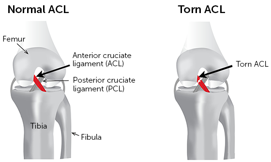
Healthy ACL (left) and Unhealthy ACL (right). Source: click here
MR images are usually taken from three basic planes, but the ACL rupture is most visible in the sagittal plane, in the few central images that target the depth of the ACL’s location. The graphic below shows the same slice of the knee in all three planes, and it can be seen that the sagittal image clearly indicates the ACL (in this case, it’s a healthy one). Because of that, we built our dataset using the images from the sagittal plane only.
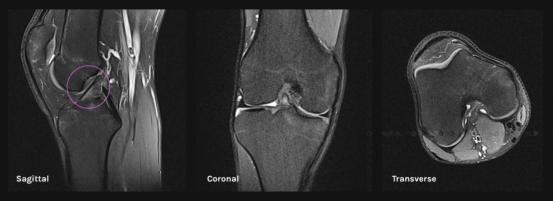
ACL preview in three basic anatomical planes
Images also vary in their scan types, a few of which do not show the ACL clearly. We filtered out those images manually when we were creating the final version of our dataset.
Dataset
Our research was performed on 761 MRI proton density fat-suppressed exams acquired from two different devices, both using 1.5T field strength. These scans were collected from General County Hospital Požega, Croatia.
When assembling our dataset, we assigned one of the following labels to each of the ACL scans:
| Label | Condition | # |
|---|---|---|
| 0 | Healthy | 462 |
| 1 | Minor Strain | 88 |
| 2 | Partially Ruptured or Strain | 59 |
| 3 | Completely Ruptured | 152 |
| TOTAL: | 761 |
The following figure shows some sample images from the dataset used for healthy and unhealthy knee images:
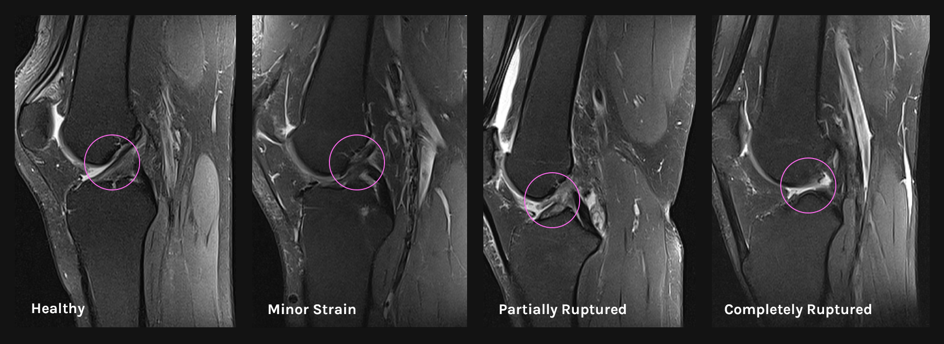
Visualization of different ACL conditions
Model Performance
The performance of our network was demonstrated via the following measures:
Research
Our goal was to take our theoretical knowledge and produce a system for classification of orthopedics MRI, focusing on knee scans, using ML techniques. In cooperation with Department of Mathematics (University of Osijek, Croatia), we started our research by following some of the standard practices in machine learning:
Choosing first model
We started following the approach similar to the research done by [Stanford ML Group] (https://stanfordmlgroup.github.io/): using the MRNet architecture that is made of the first few layers of AlexNet pre-trained on the ImageNet dataset. The diagram below, taken from Stanford’s paper illustrates the MRNet architecture:
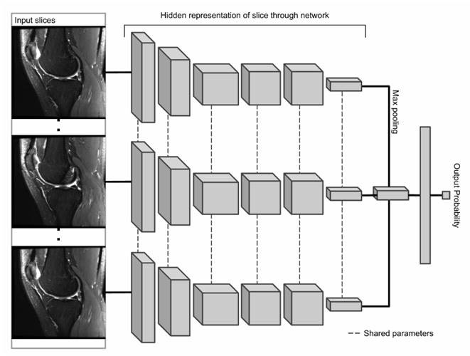
The MRNet architecture
Hyperparameter tuning
Neural networks have many variables, also known as “hyperparameters”, that need to be regulated to obtain optimal performance during the classification process. So, to get a better understanding of the correlation between the model hyperparameters and the classification results, we had to run many experiments and tune the network’s hyperparameters. While we were tweaking hyperparameters, our network reached 0.888 AUC, 83% accuracy (at most) and 18% loss (with early signs of significant overfitting on the validation set:
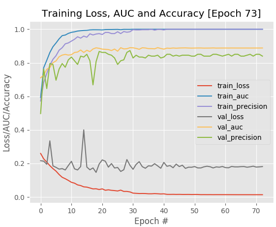
The best hyperparameter tuning experiment where we obtained 83% classification `accuracy` on our validation set (model: MRNet)
Although we didn’t succeed in boosting accuracy, as much as we wanted to (preferred: 90% and higher), we gained a better understanding of the correlations between hyperparameters and the end results.
Here are some of the hyperparameters that we adjusted in the hope to obtain a better performing network in our experiments:
- Learning rate
- Decay
- Number of epochs
- Regularization penalty
- Momentum
- Activation function
- Optimization method
- Batch size
Changing models and learning techniques
Since we could not improve the MRNet model by tweaking the hyperparameters, we tried changing the deep learning model architecture. The choice fell on the following deep learning models:
Those models are available alongside pre-trained weights, so we used them for fine-tuning, training from scratch and as arbitrary feature extractors. We thought that those models might be better in picking out the general features of the image than the older AlexNet architecture. Unfortunately, we were proven wrong. This is mostly due to models being pre-trained on the ImageNet dataset, which contains images that are quite different from the MRI scans of the ACL joint. Hence, the models were not activating correct regions of the image - regardless of the network layer at which we stop the image propagation.
The next experiments demonstrate the results we obtained while working with the VGG16 model. Other networks (VGG19, Resnet50, and SqueezeNet) failed to boost classification accuracy any higher or to decrease loss, so we classified them as a no-go for our dataset.
Fine-tuning
As can be seen in the image below, VGG16 obtained 96% accuracy and a 27% loss in the fine-tuning experiments on our validation data, which is a significant improvement in accuracy from our previous architecture.
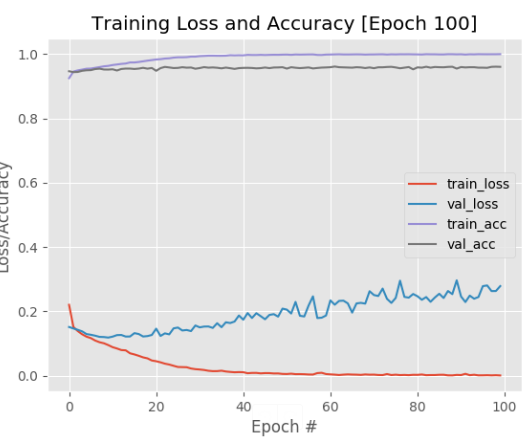
The fine-tuning experiment where we obtained 96% classification `accuracy` on our validation set (model: VGG16)
| Label | Precision | Recall | F1-score |
|---|---|---|---|
| Healthy | 0.98 | 0.99 | 0.98 |
| Minor Strain | 0.82 | 0.85 | 0.83 |
| Partially Ruptured or Strain | 0.77 | 0.51 | 0.61 |
| Completely Ruptured | 0.72 | 0.46 | 0.57 |
| Weighted Average | 0.96 | 0.96 | 0.96 |
The fine-tuning experiment metrics (model: VGG16)
However, notice how the loss from VGG16 starts to increase past epoch 20, indicating the overfitting effect. We continued experimenting with different sets of fully-connected layers by adding them to the head of the base network, but we had no luck. The network was still overfitting badly, so, in the end, we gave up fine-tuning. Retraining parts of the model was rather difficult - we spent a ton of time without improving any of the classification results.
Training network from scratch
Since features in the lower layers of networks encode the underlying representation of the feature to be detected, we decided to try training these networks from scratch. We were hoping to adopt networks to classify labels outside of what they were initially trained on.
As we feared, the network training process ended up computationally expensive and time-consuming (approximate time of computation: a couple of days using NVIDIA GTX 1080 GPU). As a side note, using just the CPU, the estimated time would be considerably longer, counting weeks (at least). Because our dataset wasn’t big enough to avoid overfitting when training the entire network from the beginning, we decided to abort this experiment as we didn’t think it would justify the long training time.
Feature Extraction
Since training the network from scratch was not an option, we wanted to try out feature extraction. That was the only reasonable remaining alternative given that we didn’t have sufficient training data and that our dataset was quite different from the original dataset (ImageNet). We still wanted to leverage the low-level features, i.e. simple concepts, picked up from the original dataset, but without the high-level data abstraction.
After a thorough investigation, the Support Vector Classifier algorithm (SVC) was shown to be best suited for the VGG16 model since it yielded the best results. As the results demonstrate (the image below), our model reached slightly lower precision (95%) compared to the fine-tuning experiment.
| Label | Precision | Recall | F1-score |
|---|---|---|---|
| Healthy | 0.98 | 0.98 | 0.98 |
| Minor Strain | 0.76 | 0.76 | 0.76 |
| Partially Ruptured or Strain | 0.53 | 0.46 | 0.49 |
| Completely Ruptured | 0.60 | 0.32 | 0.42 |
| Weighted Average | 0.95 | 0.95 | 0.95 |
Feature extraction metrics - we obtained 95% classification accuracy on our validation set (model: VGG16)
Results were a bit unexpected, so we decided to further evaluate results by using Class Activation Maps (CAM) which indicate the discriminative image regions used by our network. We found out that, even though fine-tuning had a bit higher precision, feature extraction was slightly better in discovering underlying patterns that might help with interpretation of the ACL condition. For visualization purposes, CAM filters were added on top of the images to show which areas (patterns) contributed the most to the model’s classification outcome:
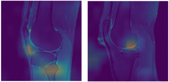
Wrong (left) and correct activations (right)
CAMs will be used in our further research and development as a primary technique to indicate problematic anatomic structures, as their output is easy to understand even for unexperienced users.
The outputs acquired with feature extraction were satisfactory, so we settled down with feature extraction as the transfer learning technique.
Performing data augmentation
The heavy overfitting to the training data led us to attempt to expand our dataset using data augmentation. The dataset was skewed heavily towards healthy diagnoses, which affected the training of the model. Our goal was to increase the number of images with unhealthy labels. However, this caused the model to heavily overfit to the training dataset as it contained a large number of similar images, and thus failed to generalize:
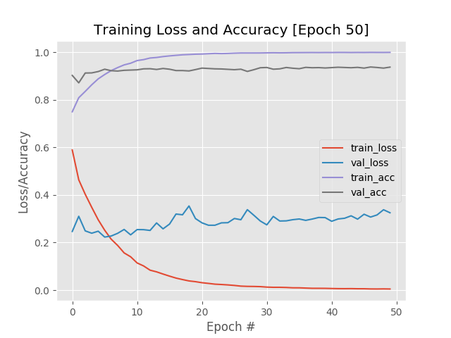
Data augmentation experiment that led to dramatic overfitting effect (model: VGG16)
Trying binary classification
Since the majority of the scans in the dataset were healthy, to improve the ratio of diagnosis labels, we combined the Minor Strain, Partially Ruptured, and Completely Ruptured labels as one Unhealthy label. This provided us with a more balanced dataset, thus slightly lowering the amount of overfitting while training the deep learning model.
| Label | Condition | # | |
|---|---|---|---|
| 0 | Healthy | 462 | |
| 1 | Unhealthy | Minor Strain | 299 |
| Partially Ruptured or Strain | |||
| Completely Ruptured | |||
| TOTAL | 761 | ||
Binary classification experiment that helped to decrease the overfitting effect (model: VGG16)
Technological problems and risks
There are several types of ML technological and related risks based on what the classification task looks like. In the table below, we’ve explained problems that we encountered throughout our experimental phases:
| Type | Description | Our Approach |
|---|---|---|
| Data Availability | Training data is not available in sufficient quantities, and almost all machine learning algorithms get significantly better results if the amount of training data from actual past cases is higher. Most medical data sets available online have only about a hundred training cases, while general-purpose data sets (e.g. ImageNet) contain millions of cases or past observations. | We tried out Data Augmentation. However, it didn’t help us because we had a pretty unbalanced dataset. |
| Quality of Data Available | In practice, compromises are often made between the duration of the scan, the signal-to-noise ratio, the number of images, and their resolution. | We manually filtered out scans if they contained too many artefacts, had inadequate resolution or if they didn’t contain objects of interest. |
| ‘Ground Truth’ | Radiologists often disagree with each other in interpreting and segmenting the same data, and although deep learning algorithms may adapt to random variability in the data to some extent due to its robustness, all ‘systematic’ deviations will affect the quality of the ML model. The anatomical structures of the human body also exhibit considerable variability, and it is, therefore, difficult to draw unambiguous conclusions. | Generally, if two radiologists disagree, a worse diagnosis will be taken into further consideration and treatment (if needed). |
| Normalization of Data Differences | Signal intensities on MR scans may also differ on the same machine, while differences in data obtained from different devices are almost inevitable. | We focused only on specific scan types: proton density fat-suppressed exams acquired from devices that are using 1.5T field strength. |
| Differences in Radiological Protocols | There is no standardized protocol for the diagnosis of individual regions, which further complicates the pre-processing process. | Radiologists have set protocols for diagnosis in place, before they started to annotate exams for the dataset. |
| Memory and Processor Requirements | The most commonly used machine learning method for processing MR scans, 3D convolutional neural networks, and several similar methods require considerable resources in terms of memory availability and processor performance. This is a challenge for scenarios where it is crucial to adapt and refine the models continually. | We performed our experiments exclusively on 2D convolutional neural networks - the reason is due to the fact that 3D networks are much more time-consuming and computationally expensive. |
| Quality of Existing Solutions and Models | Although relatively many scientific papers have been published in the past few years on the application of ML technologies and methods in processing MR results, these studies have been performed on small datasets, and their performance in real-world environments is questionable. | We used available datasets for testing purposes, and scientific papers as a metric for evaluation of our network’s performance. |
Resources
For the people just getting into ML/DL, we would recommend the “Deep Learning for Computer Vision with Python” series by Adrian Rosebrock which we found to be a great starting point.
Conclusion
Although ML techniques (DL in particular) are swiftly gaining significant impact in medical imaging, there are still many advancements that need to be made. As demonstrated by our experiments, the reliable application of DL for knee imaging faces many challenges. The most prominent issues in the process were the uneven dataset and the lack of model activation in the relevant parts of the image. The dataset problem was addressed by combining the previous three, unhealthy labels into one, creating a more balanced dataset. However, the model activation problem was improved by using segmentation which isolated the relevant underlying patterns before performing training on the deep learning model.
Stay tuned for more details about the final solution in our next post that explains various preprocessing and segmentation techniques.